Model Evaluation Using Confusion Matrix

1. Overview

“Confusion matrix sometimes also known as an error matrix, is a specific table layout that allows visualization of the performance of a supervised machine algorithm like naive Bayes, SVM, Random Forest, Logistic Regression.”

Each row of the Matrix represents the instances in a predicted class while each column represents the instances in an actual class or vice versa.

2. Confusing Matrix Layout

2.1 Binary Classification

2.1.1 Layout

2.1.2 Example

2.2 Model Evaluation parameters

2.2.1 True Positive (TP)

True Positive means the actual value and model prediction is positive.

2.2.2 False Positive (FP)

False Positive means model predict negative value as positive.

2.2.3 True Negative (TN)

True Negative means the actual value and model prediction is negative.

2.2.4 False Negative (FN)

False negative means the model predicts positive value as negative.

2.2.5 Recall, True Positive Rate, Sensitivity

Recall refers to out of total relevant documents how many are successfully retrieved. We can calculate recall using below formula.

2.2.6 Precision

Precision refers to out of retrieved documents how many are correct.

2.2.7 False Positive Rate

2.2.8 True Negative Rate

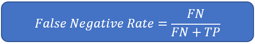
2.2.9 False Negative Rate

2.2.10 F1-score

2.2.11 Overall Accuracy

3. Development Environment

Python : 3.6.5

IDE       : Pycharm community Edition

scikit-learn : 0.20.0

matlabplot : 3.0.0

4. Example

import pandas as pd
import numpy as np
from pathlib import Path
import sklearn.datasets as skds
import matplotlib.pyplot as plt
from sklearn.metrics import confusion_matrix
from sklearn.feature_extraction.text import CountVectorizer
import itertools
"""Load text files with categories as subfolder names.
    Individual samples are assumed to be files stored a two levels folder
    structure such as the following:
        EmailSpam/
            Spam/
                file_1.txt
                file_2.txt
                ...
                file_42.txt
            ham/
                file_43.txt
                file_44.txt
                ..."""
# Source file directory
path_train = "G:\\DataSet\\DataSet\\EmailSpam\\EmailSpam"
files_train = skds.load_files(path_train, load_content=False)
label_index = files_train.target
label_names = files_train.target_names
labelled_files = files_train.filenames
data_tags = ["filename", "category", "content"]
data_list = []
# Read and add data from file to a list
i = 0
for f in labelled_files:
    data_list.append((f, label_names[label_index[i]], Path(f).read_text()))
    i += 1
# We have training data available as dictionary filename, category, data
data = pd.DataFrame.from_records(data_list, columns=data_tags)
# lets take 80% data as training and remaining 20% for test.
train_size = int(len(data) * .4)
train_posts = data['content'][:train_size]
train_tags = data['category'][:train_size]
train_files_names = data['filename'][:train_size]
test_posts = data['content'][train_size:]
test_tags = data['category'][train_size:]
test_files_names = data['filename'][train_size:]
print("Training Set Size "+str(len(train_posts)))
print("Testing Set Size "+str(len(test_posts)))

# https://www.kaggle.com/adamschroeder/countvectorizer-tfidfvectorizer-predict-comments
# https://www.opencodez.com/python/text-classification-using-keras.htm
vectorizer = CountVectorizer(stop_words='english',max_features=40)
X_train = vectorizer.fit_transform(train_posts)
X_test = vectorizer.transform(test_posts)
from sklearn.naive_bayes import MultinomialNB
clf = MultinomialNB()
clf.fit(X_train, train_tags)
print("start applying on testing data set")
predictions = clf.predict(X_test)
print("Model applied on testing data set")
# Compute confusion matrix
cnf_matrix = confusion_matrix(test_tags, predictions)
np.set_printoptions(precision=2)
class_names = ["ham", "spam"]

# Plot non-normalized confusion matrix
def plot_confusion_matrix(cm, classes,
                          title='Confusion matrix',
                          cmap=plt.cm.Blues):
    """
    This function prints and plots the confusion matrix.
    Normalization can be applied by setting `normalize=True`.
    """
    plt.figure()
    print("Normalized confusion matrix")
    print(cm)
    plt.imshow(cm, interpolation='nearest', cmap=cmap)
    plt.title(title)
    plt.colorbar()
    tick_marks = np.arange(len(classes))
    plt.xticks(tick_marks, classes, rotation=45)
    plt.yticks(tick_marks, classes)
    fmt = 'd'
    thresh = cm.max() / 2.
    for i, j in itertools.product(range(cm.shape[0]), range(cm.shape[1])):
        plt.text(j, i, format(cm[i, j], fmt),
                 horizontalalignment="center",
                 color="white" if cm[i, j] > thresh else "black")
    plt.ylabel('True label')
    plt.xlabel('Predicted label')
    plt.tight_layout()
    plt.show()

plot_confusion_matrix(cnf_matrix, classes=class_names,
                      title='Confusion matrix')
print("complete")

5. Output

Here is the output of MultiNomial Naive Bayes Classification model confusion matrix on our test datasets. From this output, we can make the decision of how our model is performed.

6. Conclusion

In this article, we have discussed the basic layout of the binary classification confusion matrix and its layout example. Precision, recall and other model evaluation parameters along formulas and at last complete example of how to fit MultiNomial Navie Bayes model and plot confusion matrix plot using matplotlib.

7. References

Refer below links for more details.

• scikit-learn
• Naive Bayes
• Data Frame
• Naive Bayes Text Classification Example
• Machine Learning General Steps

8. Source Code

Model Evaluation Using ConfusionMatrix Example

You can also download source code of Model Evaluation Using Confusion Matrix and other useful examples from our git repository.